
Surface Reflectance and NDVI Fusion#
This notebook will demonstrate how to access Hydrosat’s daily surface reflectance data which is constructed from a fused output of Sentinel-2 and MODIS MCD43A4 surface reflectance products. We will show:
Accessing the fused and input surface reflectance data through the Fusion Hub STAC API
Sampling the data to produce NDVI for a point location
Comparing the fused NDVI and source NDVI for Sentinel-2 and MCD43A4 surface reflectance products
Let’s import the required packages
import json
import pystac
from pystac_client import Client
from pprint import pprint
from pyproj.crs import CRS

import xarray as xr
import rioxarray as rxr
import rasterio as rio

from matplotlib import pyplot as plt
import numpy as np

import pandas as pd
from FH_Hydrosat import FH_Hydrosat

import base64

from shapely.geometry import Point, box
from datetime import datetime as DT
# import geopandas as gpd
This next cell opens a file creds.json which you will need to create in the same directory as the notebook. The format of the file should be:
{
"username":"your_username",
"password":"your_password"
}
and you have updated with your username and password.
with open('creds.json') as f:
    creds = json.loads(f.read())
This next cell will endecode the username:password combination and use it to authorize access to the STAC API given by the cat_url endpoint.
userpass = f"{creds['username']}:{creds['password']}"
b64 = base64.b64encode(userpass.encode()).decode()
headers = {'Authorization':'Basic ' + b64}

cat_url = 'https://stac.hydrosat.com'
catalog = Client.open(cat_url, headers)
We’ll search for data in the starfm_predictions_modis_s2 and prepped_inputs_s2 collections which intersect a point location between a start date and an end date and print out the number of items. Note that in this example, the prepped_inputs_s2 collection contains surface reflectance data constructed from 30-day median composites of Sentinel-2 scenes.
NOTE: Accessing a years worth of data in this example may result in slow notebook performance. If you are noticing slow performance, adjust the date range to something more manageable but within the year 2021.
bbox = [-120.5141,36.4316,-120.4541,36.4827]

start_date = "2021-01-01T00:00:00Z"
end_date = "2021-12-31T23:59:59Z"
coll = ""

#########################################################################
search = catalog.search(
    collections = [f"starfm_predictions_modis_s2{coll}"],
    bbox=bbox,
    datetime = [start_date, end_date],
    max_items = 500
)

ts_items = search.get_all_items()
print(f'number of sharpened SR items: {len(ts_items)}')

search = catalog.search(
    collections = [f"prepped_inputs_s2{coll}"],
    bbox=bbox,
    datetime = [start_date, end_date],
    max_items = 500
)

s2_items = search.get_all_items()
print(f'number of source SR items: {len(s2_items)}')
C:\software\Anaconda3\envs\hydrosat\lib\site-packages\pystac_client\item_search.py:850: FutureWarning: get_all_items() is deprecated, use item_collection() instead.
  warnings.warn(
number of sharpened SR items: 291
number of source SR items: 36
To see how the fused surface reflectance items are organized we can print out the asset names from one of the items in ts_items
ts_items[0].to_dict()['assets'].keys()
dict_keys(['combined_qa', 'surface_reflectance_blue', 'valid_data_mask', 'surface_reflectance_green', 'surface_reflectance_red', 'surface_reflectance_nir', 'preview', 'thumbnail'])
Let’s create objects to hold the Red and NIR assets from each item in the time series. We can look at a full time series of the sharpened NDVI items by sampling the point location using functionality included in FH_Hydrosat.py.
from FH_Hydrosat import FH_Hydrosat
point_wgs84 = Point(box(*bbox).centroid.x, box(*bbox).centroid.y)
res_red_full = FH_Hydrosat(ts_items, asset='surface_reflectance_red')
res_nir_full = FH_Hydrosat(ts_items, asset='surface_reflectance_nir')

red_ts = res_red_full.point_time_series_from_items(point_wgs84, tol=40, nproc=6)
red_dt = res_red_full.datetime

nir_ts = res_nir_full.point_time_series_from_items(point_wgs84, tol=40, nproc=6)
nir_dt = res_nir_full.datetime
using 6 processes to sample 291 assets
using 6 processes to sample 291 assets
We can construct the NDVI time series using the well known NDVI equation and the associated datetimes.
$ NDVI = \frac{NIR - RED}{NIR + RED} $
ndvi_ts = (np.array(nir_ts) - np.array(red_ts)) / (np.array(nir_ts) + np.array(red_ts))
ndvi_dt = nir_dt # same as either nir or red
We’ll add the time series data and dates to a pandas dataframe to help with plotting.
ndvi_df = pd.DataFrame({'ndvi': ndvi_ts,
                          'datetime': pd.to_datetime(ndvi_dt)}).sort_values(by='datetime')
ndvi_df['date'] = [t.to_pydatetime().strftime('%Y-%m-%d') for t in ndvi_df['datetime']]

ndvi_df = ndvi_df.set_index(ndvi_df['date'])
ndvi_df['color'] = 'blue' # color to plot with
The STARFM items do not include the source items from Sentinel-2 which are needed to fill in the remainder of the time series. We’ll sample the Sentinel-2 items for the Red band and NIR band 8A. The data in prepped_inputs_s2 has the following band mapping:
prepped_inputs_s2 band index |
Sentinel-2 band |
|---|---|
0 |
B02 |
1 |
B03 |
2 |
B04 |
3 |
B05 |
4 |
B06 |
5 |
B07 |
6 |
B8A |
7 |
B11 |
8 |
B12 |
Here is a visual of the spectrum covered by the bands represented in this product (https://sentinels.copernicus.eu/web/sentinel/user-guides/sentinel-2-msi/resolutions/spatial).


# sample the s2 items
s2_res = FH_Hydrosat(s2_items, asset='surface_reflectance')
s2_red_ts = s2_res.point_time_series_from_items(point_wgs84, tol=40, nproc=6, band=2)
s2_nir_ts = s2_res.point_time_series_from_items(point_wgs84, tol=40, nproc=6, band=6)
s2_dt = s2_res.datetime
using 6 processes to sample 36 assets
using 6 processes to sample 36 assets
Similar to above, we’ll calculate NDVI using the NIR and RED time series
s2_ndvi_ts = (np.array(s2_nir_ts) - np.array(s2_red_ts)) / (np.array(s2_nir_ts) + np.array(s2_nir_ts))

s2_ndvi_df = pd.DataFrame({'ndvi': s2_ndvi_ts,
                          'datetime': pd.to_datetime(s2_dt)}).sort_values(by='datetime')
s2_ndvi_df['date'] = [t.to_pydatetime().strftime('%Y-%m-%d') for t in s2_ndvi_df['datetime']]

s2_ndvi_df = s2_ndvi_df.set_index(s2_ndvi_df['date'])
s2_ndvi_df['color'] = 'red'
Next, we’ll join the two dataframes together to complete the time series.
full_ndvi_df = pd.merge(ndvi_df.drop('date', axis=1), s2_ndvi_df.drop('date', axis=1), left_index=True, right_index=True, how='outer')
full_ndvi_df = pd.concat((ndvi_df, s2_ndvi_df), axis=0)
full_ndvi_df.sort_index(inplace=True)
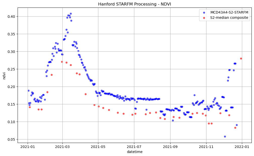
We’ll plot the fused NDVI and the Sentinel-2 NDVI as two different colors: red and blue, respectively.
fig, ax = plt.subplots()
for i in full_ndvi_df.color.unique():
    df_color = full_ndvi_df[full_ndvi_df.color==i]
    df_color.plot.scatter(x='datetime', y='ndvi', ax=ax, c=i, label=df_color.color.iloc[0],
                         grid=True, alpha=0.6, figsize=(12,7))


ax.set_title('Hanford STARFM Processing - NDVI');
plt.legend(['MCD43A4-S2-STARFM', 'S2-median composite']);
blue
red
Next, we will check the MCD43A4 data which was used as an input to produce the fused surface reflectance data. Let’s retrieve that data from the STAC API
search = catalog.search(
    collections = [f"prepped_inputs_mcd43a4{coll}"],
    bbox=bbox,
    datetime = [start_date, end_date],
    max_items = 500
)

mcd_items = search.get_all_items()
print(f'number of source MODIS SR items: {len(mcd_items)}')
C:\software\Anaconda3\envs\hydrosat\lib\site-packages\pystac_client\item_search.py:850: FutureWarning: get_all_items() is deprecated, use item_collection() instead.
  warnings.warn(
number of source MODIS SR items: 354
We’ll sample the MCD43 items the same as before, but using the correct bands for MCD43A4. See this table for the band mappings (https://eos.com/find-satellite/modis-mcd43a4/). We will use bands 1 and 2, which are indexed by 0 and 1.
# sample the MCD43 items
mcd_res = FH_Hydrosat(mcd_items, asset='surface_reflectance')
mcd_red_ts = mcd_res.point_time_series_from_items(point_wgs84, tol=1000, nproc=6, band=0)
mcd_nir_ts = mcd_res.point_time_series_from_items(point_wgs84, tol=1000, nproc=6, band=1)
mcd_dt = mcd_res.datetime
using 6 processes to sample 354 assets
using 6 processes to sample 354 assets
As before, we will construct the NDVI series and pass it to a DataFrame, this time specifying cyan in the color column.
mcd_ndvi_ts = (np.array(mcd_nir_ts) - np.array(mcd_red_ts)) / (np.array(mcd_nir_ts) + np.array(mcd_nir_ts))

mcd_ndvi_df = pd.DataFrame({'ndvi': mcd_ndvi_ts,
                          'datetime': pd.to_datetime(mcd_dt)}).sort_values(by='datetime')
mcd_ndvi_df['date'] = [t.to_pydatetime().strftime('%Y-%m-%d') for t in mcd_ndvi_df['datetime']]

mcd_ndvi_df = mcd_ndvi_df.set_index(mcd_ndvi_df['date'])
mcd_ndvi_df['color'] = 'cyan'
full_ndvi_df2 will hold the fused NDVI, Sentinel-2 NDVI, and MCD43A4 NDVI in a single DataFrame.
full_ndvi_df2 = pd.concat((ndvi_df, s2_ndvi_df, mcd_ndvi_df), axis=0)
full_ndvi_df2.sort_index(inplace=True)
Finally, we plot them all together.
fig, ax = plt.subplots()
for i in full_ndvi_df2.color.unique():
    df_color = full_ndvi_df2[full_ndvi_df2.color==i]
    df_color.plot.scatter(x='datetime', y='ndvi', ax=ax, c=i, label=df_color.color.iloc[0],
                         grid=True, alpha=0.6, figsize=(12,7))


ax.set_title('Hanford STARFM Processing - NDVI');
plt.legend(['MCD43A4-S2-STARFM', 'MCD43A4', 'S2 median composite']);
blue
cyan
red
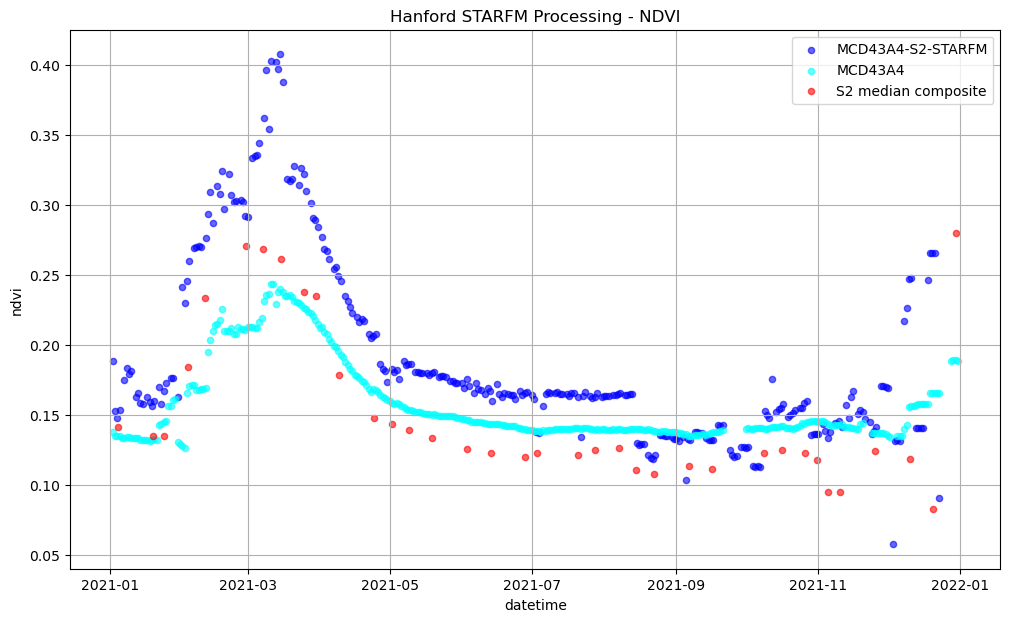
There are some obvious differences in the NDVI plots above, namely that the NDVI calculated from the MODIS MCD43A4 product is often higher than the Sentinel-2 data. One difference is the MCD43A4 product is adjusted for different viewing angles through Bidirectional-Reflectance Distribution Function (BRDF), and is a “best-of” product constructed from daily observations over the course of 16 days. Addtionally, there are spectral bandwidth differences in the bands used to construct NDVI between Sentinel-2 and the MODIS MCD43A4 surface reflectance products (shown below). The MODIS product provides the daily surface reflectance information to the fusion process and the fused NDVI values will track those values.
(band information retrieved from https://landsat.usgs.gov/spectral-characteristics-viewer)