Fusion Hub Data Quick-Start

This notebook demonstrates the process of:

• Searching a collection to intersect a point location between a start data and end date

• Converting the search result to an xarray DataArray

• Subsetting the DataArray to a geometry

• Plotting the time series in a grid

• Extracting data from a point location

• Reducing the data within a geometry

• Downloading a file based on valid data percentage

• Downloading multiple files

• Removing data entries based on some condition

• Creating matplotlib animations

import json
import requests
import pystac
from pystac_client import Client
from pprint import pprint

from botocore.exceptions import ClientError
from shapely.geometry import box, mapping, Point, Polygon
from pyproj.crs import CRS
import geopandas as gpd

import xarray as xr
import rioxarray as rxr
import rasterio as rio

from matplotlib import pyplot as plt
import numpy as np

import os
import base64

If you see ERROR 1: PROJ: proj_create_from_database: Open of /opt/conda/share/proj failed, do not fret, and proceed.

This next cell opens a file creds.json which you will need to create in the same directory as the notebook. The format of the file should be:

{
"username":"your_username",
"password":"your_password"
}

and you have updated with your username and password.

with open('creds.json') as f:
    creds = json.loads(f.read())
    

This next cell will endecode the username:password combination and use it to authorize access to the STAC API given by the cat_url endpoint.

userpass = f"{creds['username']}:{creds['password']}"
b64 = base64.b64encode(userpass.encode()).decode()
headers = {'Authorization':'Basic ' + b64}

cat_url = 'https://fusion-stac.hydrosat.com'
catalog = Client.open(cat_url, headers)

We’ll search for data in the starfm_predictions_modis_landsat and pydms_sharpened_landsat collections which intersect a point location between a start date and an end date and print out the number of items.

geom = {'type': 'Point', 'coordinates': [-120.21102905273436,36.535019209789]} # Point for Hanford, CA, USA

collections = ["starfm_predictions_modis_landsat", "pydms_sharpened_landsat"]
start_date = "2021-08-17T00:00:00Z"
end_date = "2021-10-30T00:00:00Z"

search = catalog.search(
    collections = collections,
    intersects = geom,
    datetime = [start_date, end_date],
    max_items = 500
)

# items = list(search.items()) # for pystac-client >= 0.4.0
items = list(search.get_all_items()) # for pystac-client < 0.4.0
items.reverse() # make the results ascending in time
len(items)

65

This next cell will determine if the data returned covers more than a single MGRS tile. If there is, choose one of the tiles to subset the list of returned items.

mgrs_tiles = []
for i in items:
    for l in i.to_dict()['links']:
        if 'element84' in l['href']:
            mgrs_tiles.append(l['href'].split(r'/')[-1].split('_')[1])
print(f'number of tiles in query: {len(set(mgrs_tiles))}, {set(mgrs_tiles)}')

# if there is more than one tile, uncomment and execute this next line to choose the MGRS tile you are interested in
# items = [i for i in items if mgrs_tiles[0] in i.id]

number of tiles in query: 1, {'10SGF'}

Now we’ll pass the first 25 items to the FH_Hydrosat class and stack the items into an xarray DataArray. We’ll print out the DataArray to get a summary of its contents.

from FH_Hydrosat import FH_Hydrosat
res = FH_Hydrosat(items[:25])
stacked_res = res.stack()
stacked_res.ds.sortby('time')

<xarray.DataArray (time: 25, band: 1, y: 5490, x: 5490)>
dask.array<concatenate, shape=(25, 1, 5490, 5490), dtype=float32, chunksize=(1, 1, 2048, 2048), chunktype=numpy.ndarray>
Coordinates:
  * band         (band) int32 1
  * x            (x) float64 7e+05 7e+05 7e+05 ... 8.097e+05 8.097e+05 8.098e+05
  * y            (y) float64 4.1e+06 4.1e+06 4.1e+06 ... 3.99e+06 3.99e+06
    spatial_ref  int32 0
  * time         (time) object 2021-08-17T11:59:59.500000+00:00 ... 2021-09-1...
Attributes:
    _FillValue:    nan
    scale_factor:  1.0
    add_offset:    0.0

xarray.DataArray

• time: 25
• band: 1
• y: 5490
• x: 5490

• dask.array<chunksize=(1, 1, 2048, 2048), meta=np.ndarray>

  Array Chunk Bytes 2.81 GiB 16.00 MiB Shape (25, 1, 5490, 5490) (1, 1, 2048, 2048) Count 700 Tasks 225 Chunks Type float32 numpy.ndarray

• Coordinates: (5)
  • band
    (band)
    int32
    1

    array([1])

  • x
    (x)
    float64
    7e+05 7e+05 ... 8.097e+05 8.098e+05

    array([699970., 699990., 700010., ..., 809710., 809730., 809750.])

  • y
    (y)
    float64
    4.1e+06 4.1e+06 ... 3.99e+06

    array([4100030., 4100010., 4099990., ..., 3990290., 3990270., 3990250.])

  • spatial_ref
    ()
    int32
    0

    crs_wkt :

    PROJCS["WGS 84 / UTM zone 10N",GEOGCS["WGS 84",DATUM["WGS_1984",SPHEROID["WGS 84",6378137,298.257223563,AUTHORITY["EPSG","7030"]],AUTHORITY["EPSG","6326"]],PRIMEM["Greenwich",0,AUTHORITY["EPSG","8901"]],UNIT["degree",0.0174532925199433,AUTHORITY["EPSG","9122"]],AUTHORITY["EPSG","4326"]],PROJECTION["Transverse_Mercator"],PARAMETER["latitude_of_origin",0],PARAMETER["central_meridian",-123],PARAMETER["scale_factor",0.9996],PARAMETER["false_easting",500000],PARAMETER["false_northing",0],UNIT["metre",1,AUTHORITY["EPSG","9001"]],AXIS["Easting",EAST],AXIS["Northing",NORTH],AUTHORITY["EPSG","32610"]]

    semi_major_axis :

    6378137.0

    semi_minor_axis :

    6356752.314245179

    inverse_flattening :

    298.257223563

    reference_ellipsoid_name :

    WGS 84

    longitude_of_prime_meridian :

    0.0

    prime_meridian_name :

    Greenwich

    geographic_crs_name :

    WGS 84

    horizontal_datum_name :

    World Geodetic System 1984

    projected_crs_name :

    WGS 84 / UTM zone 10N

    grid_mapping_name :

    transverse_mercator

    latitude_of_projection_origin :

    0.0

    longitude_of_central_meridian :

    -123.0

    false_easting :

    500000.0

    false_northing :

    0.0

    scale_factor_at_central_meridian :

    0.9996

    spatial_ref :

    PROJCS["WGS 84 / UTM zone 10N",GEOGCS["WGS 84",DATUM["WGS_1984",SPHEROID["WGS 84",6378137,298.257223563,AUTHORITY["EPSG","7030"]],AUTHORITY["EPSG","6326"]],PRIMEM["Greenwich",0,AUTHORITY["EPSG","8901"]],UNIT["degree",0.0174532925199433,AUTHORITY["EPSG","9122"]],AUTHORITY["EPSG","4326"]],PROJECTION["Transverse_Mercator"],PARAMETER["latitude_of_origin",0],PARAMETER["central_meridian",-123],PARAMETER["scale_factor",0.9996],PARAMETER["false_easting",500000],PARAMETER["false_northing",0],UNIT["metre",1,AUTHORITY["EPSG","9001"]],AXIS["Easting",EAST],AXIS["Northing",NORTH],AUTHORITY["EPSG","32610"]]

    GeoTransform :

    699960.0 20.0 0.0 4100040.0 0.0 -20.0

    array(0)

  • time
    (time)
    object
    2021-08-17T11:59:59.500000+00:00...

    array([Timestamp('2021-08-17 11:59:59.500000+0000', tz='UTC'),
           Timestamp('2021-08-18 11:59:59.500000+0000', tz='UTC'),
           Timestamp('2021-08-19 11:59:59.500000+0000', tz='UTC'),
           Timestamp('2021-08-20 11:59:59.500000+0000', tz='UTC'),
           Timestamp('2021-08-21 18:40:16.415650+0000', tz='UTC'),
           Timestamp('2021-08-22 11:59:59.500000+0000', tz='UTC'),
           Timestamp('2021-08-23 11:59:59.500000+0000', tz='UTC'),
           Timestamp('2021-08-24 11:59:59.500000+0000', tz='UTC'),
           Timestamp('2021-08-25 11:59:59.500000+0000', tz='UTC'),
           Timestamp('2021-08-26 11:59:59.500000+0000', tz='UTC'),
           Timestamp('2021-08-27 11:59:59.500000+0000', tz='UTC'),
           Timestamp('2021-08-28 11:59:59.500000+0000', tz='UTC'),
           Timestamp('2021-08-29 11:59:59.500000+0000', tz='UTC'),
           Timestamp('2021-08-30 18:33:56.253740+0000', tz='UTC'),
           Timestamp('2021-08-31 11:59:59.500000+0000', tz='UTC'),
           Timestamp('2021-09-01 11:59:59.500000+0000', tz='UTC'),
           Timestamp('2021-09-02 11:59:59.500000+0000', tz='UTC'),
           Timestamp('2021-09-03 11:59:59.500000+0000', tz='UTC'),
           Timestamp('2021-09-04 11:59:59.500000+0000', tz='UTC'),
           Timestamp('2021-09-05 11:59:59.500000+0000', tz='UTC'),
           Timestamp('2021-09-06 18:40:21.164950+0000', tz='UTC'),
           Timestamp('2021-09-07 11:59:59.500000+0000', tz='UTC'),
           Timestamp('2021-09-08 11:59:59.500000+0000', tz='UTC'),
           Timestamp('2021-09-09 11:59:59.500000+0000', tz='UTC'),
           Timestamp('2021-09-10 11:59:59.500000+0000', tz='UTC')], dtype=object)

• Attributes: (3)

  _FillValue :

  nan

  scale_factor :

  1.0

  add_offset :

  0.0

ds = stacked_res.ds.sortby('time')

The DataArray is quite large if we try to access all of the data. For ease of computation, we’ll subset the DataArray by a polygon, which will be generated by creating a rectangular buffer around the point location by 1km on either side.

p_geom = Point(geom['coordinates'][0], geom['coordinates'][1])
point_df = gpd.GeoDataFrame({'geometry':[p_geom]}, crs=CRS.from_epsg(4326))

raster_crs = CRS.from_wkt(ds.spatial_ref.crs_wkt)
buffer_dist = 1000 # 1km in local UTM zone
poly_df = point_df.to_crs(raster_crs).buffer(buffer_dist, cap_style = 3) # square buffer

Let’s plot the polygon on a Folium map so we can see where we are extracting the data

import folium 

# Use WGS 84 (epsg:4326) as the geographic coordinate system
df = gpd.GeoDataFrame(poly_df.to_crs(epsg=4326))

m = folium.Map(location=[p_geom.y, p_geom.x], zoom_start=13, tiles='CartoDB positron')

# add the polygon and centroid
for _, r in df.iterrows():
    # Without simplifying the representation of each polygon,
    # the map might not be displayed
    #sim_geo = gpd.GeoSeries(r['geometry']).simplify(tolerance=0.001)
    sim_geo = r[0].simplify(tolerance=0.001)
    geo_j = gpd.GeoSeries(sim_geo).to_json()
    geo_j = folium.GeoJson(data=geo_j,
                           style_function=lambda x: {'fillColor': 'orange'})
    
    geo_j.add_to(m)
    
    lat = sim_geo.centroid.y
    lon = sim_geo.centroid.x
    folium.Marker(location=[lat, lon]).add_to(m)
    
m

Make this Notebook Trusted to load map: File -> Trust Notebook

Now let’s clip the dataset with the geometry using rioxarray’s rio utility package

from FH_Hydrosat import FH_StackedDataset

# clip the raster dataset and cast to a class with slightly more functions
clipped = FH_StackedDataset(ds.rio.clip(poly_df.geometry))
ds_clip = clipped.ds

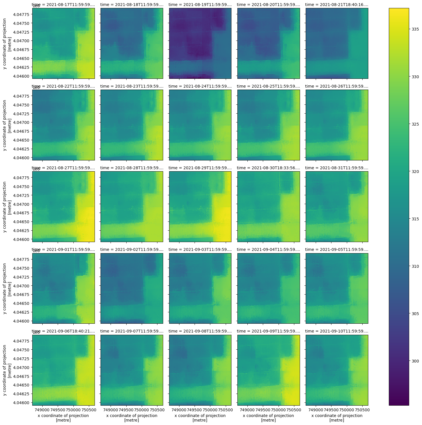
Now that we have a smaller DataArray, let’s plot the contents according to the time dimension using xarray’s plot utility.

ds_clip.plot(x='x', y='y', col='time', col_wrap=5);

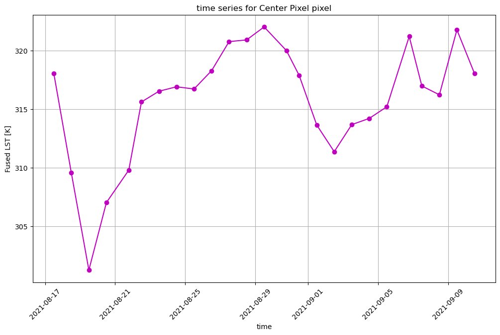
Plot a time series for the point location

With the same DataArray, we can extract the pixel values which intersect a point location. Let’s use the same point location we used to search the STAC catalog and plot it.

centroid = poly_df.geometry[0].centroid
set_x, set_y, pixtype = (centroid.x, centroid.y, 'Center Pixel') # change 'Center Pixel' for plot title

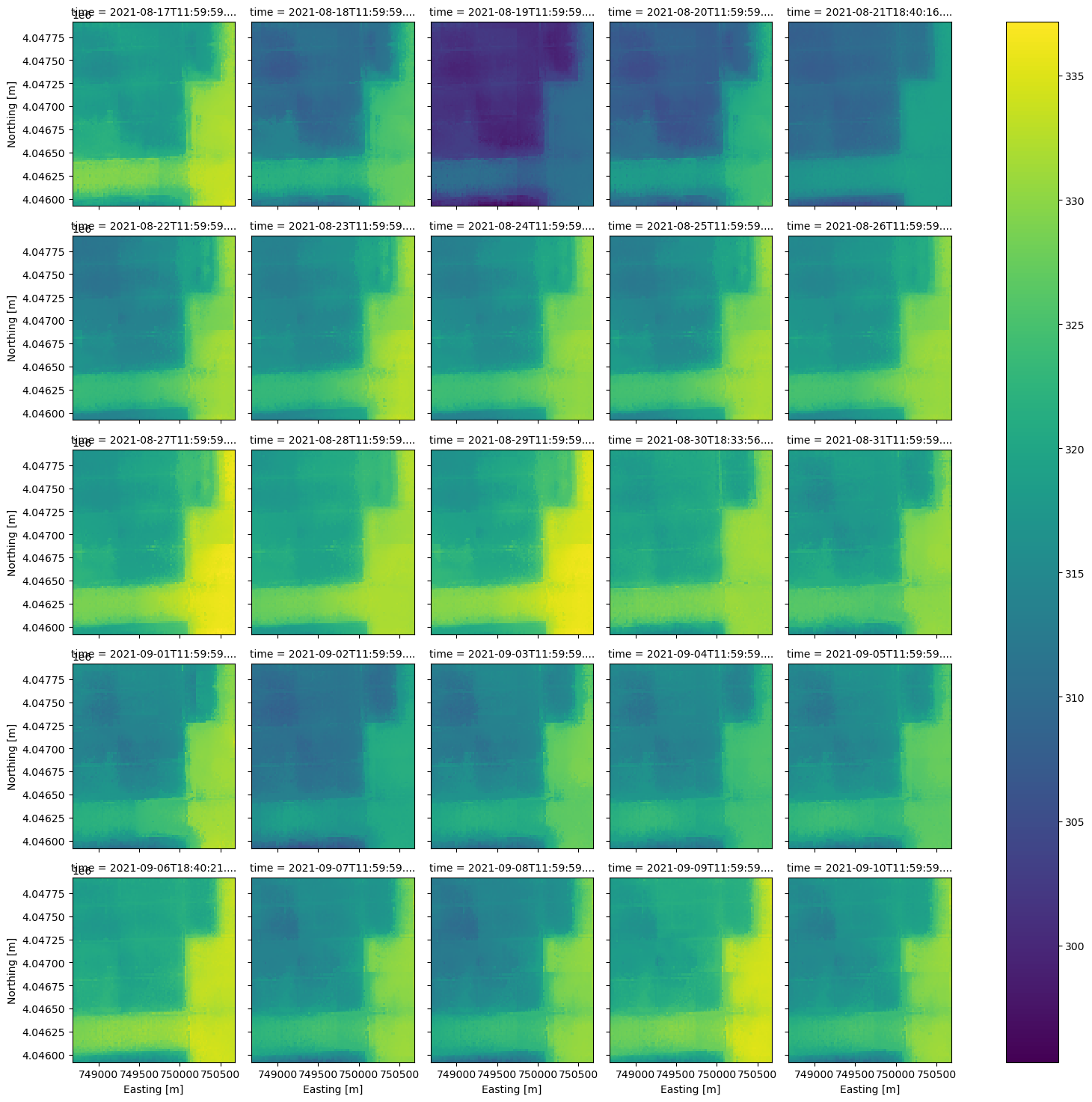
ax = ds_clip.plot(x='x', y='y', col='time', col_wrap=5)
ax.set_xlabels('Easting [m]')
ax.set_ylabels('Northing [m]')
ax.map(lambda: plt.plot(set_x, set_y, markersize=20, marker=".", color="m"))
plt.show()


ax = ds_clip.isel(band=0).sel(x=set_x, y=set_y, method='nearest', tolerance=20).plot(marker='o', c='m', figsize=(12,7))
plt.title(f'time series for {pixtype} pixel')
plt.grid(True)
plt.ylabel('Fused LST [K]')
plt.xticks(rotation=45)
plt.show()

C:\software\Anaconda3\envs\hydrosat\lib\site-packages\xarray\core\indexes.py:234: FutureWarning: Passing method to Float64Index.get_loc is deprecated and will raise in a future version. Use index.get_indexer([item], method=...) instead.
  indexer = self.index.get_loc(
C:\software\Anaconda3\envs\hydrosat\lib\site-packages\xarray\core\indexes.py:234: FutureWarning: Passing method to Float64Index.get_loc is deprecated and will raise in a future version. Use index.get_indexer([item], method=...) instead.
  indexer = self.index.get_loc(

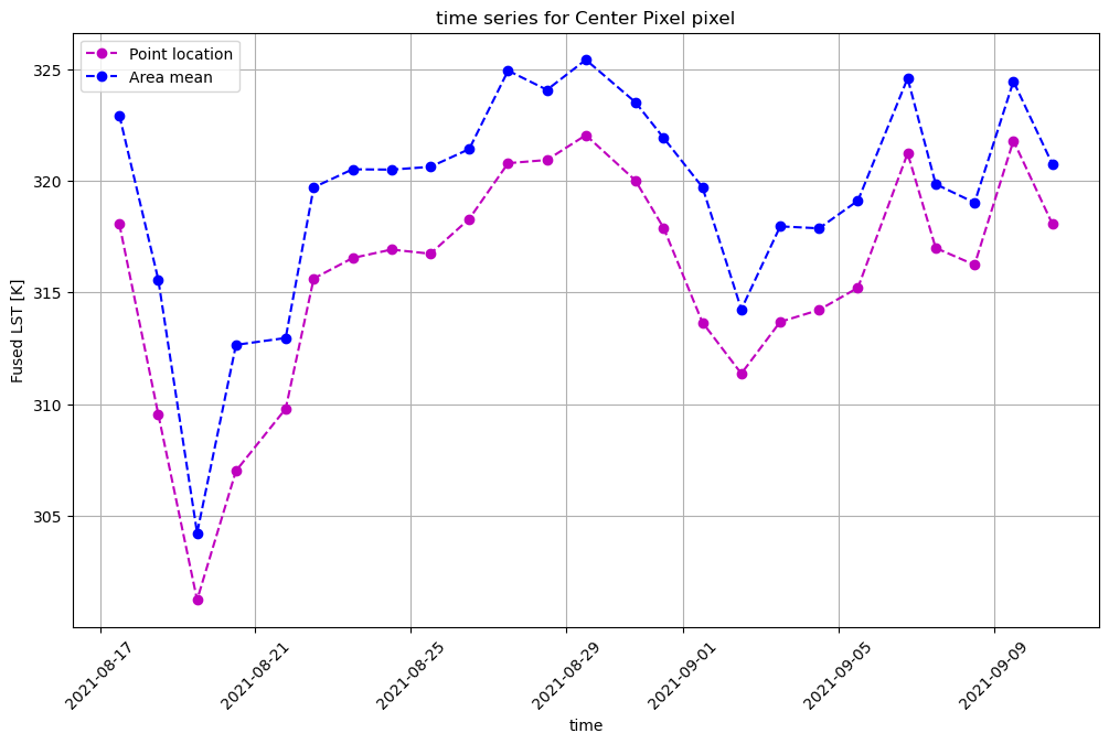
Similarly, we can reduce the area within the subsetting geometry to the mean value, and plot against the time series for the point location.

ax = ds_clip.plot(x='x', y='y', col='time', col_wrap=5)
ax.set_xlabels('Easting [m]')
ax.set_ylabels('Northing [m]')
ax.map(lambda: plt.plot(set_x, set_y, markersize=20, marker=".", color="m"))
plt.show()


ax = ds_clip.isel(band=0).sel(x=set_x, y=set_y, method='nearest', tolerance=20).plot(linestyle='--', marker='o', c='m', label='Point location', figsize=(12,7))
ax = ds_clip.isel(band=0).mean(dim=('x', 'y')).plot(linestyle='--', marker='o', c='b', label='Area mean')
plt.title(f'time series for {pixtype} pixel')
plt.legend()
plt.grid(True)
plt.ylabel('Fused LST [K]')
plt.xticks(rotation=45)
plt.show()

C:\software\Anaconda3\envs\hydrosat\lib\site-packages\xarray\core\indexes.py:234: FutureWarning: Passing method to Float64Index.get_loc is deprecated and will raise in a future version. Use index.get_indexer([item], method=...) instead.
  indexer = self.index.get_loc(
C:\software\Anaconda3\envs\hydrosat\lib\site-packages\xarray\core\indexes.py:234: FutureWarning: Passing method to Float64Index.get_loc is deprecated and will raise in a future version. Use index.get_indexer([item], method=...) instead.
  indexer = self.index.get_loc(

download a single file

# find which file has the most data in it
max_data_idx = np.argmax(ds_clip.count(dim=('x', 'y', 'band')).values)

outfile = f'./{os.path.basename(res.item_desc[max_data_idx])}'
print(outfile, os.path.exists(outfile))

res.download_single_asset(max_data_idx)

print(outfile, os.path.exists(outfile))

./10SGF_pred_20210817_from_20210814_using_MODIS_Landsat.tif True
./10SGF_pred_20210817_from_20210814_using_MODIS_Landsat.tif True

download multiple files, since there a few scenes that have full coverage for the AOI

# download the items above which correspond to items 2,5,6, and 10
# using the download_multiple_assets() function
res.download_multiple_assets([2,5,6,10])

using 2 processes to download 4 assets

make an animation from the full set of data

If you see Javascript Error: IPython is not defined or MovieWriter ffmpeg unavailable; using Pillow instead, do not fret, and proceed.

from IPython.display import HTML

# switch plotting to allow for animations
%matplotlib notebook 

# use the create_animation() function.
# display the animation with HTML display
ani = clipped.create_animation(save_ani=True, vmin=300, vmax=350)
HTML(ani.to_jshtml())

Once Loop Reflect

drop files with data less than 50% coverage

Sometimes the data will have low coverage due to cloud cover or invalid pixels in the input data products. Let’s remove them from the dataset using the remove_below_data_perc() function, plot them, and create an animation.

# to switch back and allow xarray plots
%matplotlib inline 

more_data = FH_StackedDataset(clipped.remove_below_data_perc(clipped.ds, 0.5))
ax = more_data.ds.plot(x='x', y='y', col='time', col_wrap=5)
ax.set_xlabels('Easting [m]')
ax.set_ylabels('Northing [m]')
plt.show()

 # switch back to allow animation
%matplotlib notebook
ani = more_data.create_animation(save_ani=True, vmin=300, vmax=350, anipath='more_data.gif')
HTML(ani.to_jshtml())

Once Loop Reflect

You may notice that the animation plays with the most recent date in the data stack first, and then ascending. To reverse the order to descending from the last date in the dataset, use an xarray call to reverse the time dimension on the dataset.

# reverse the order
more_data_rev = FH_StackedDataset(more_data.ds.sortby('time', ascending=False))
ani = more_data_rev.create_animation(save_ani=True, vmin=300, vmax=350, anipath='more_data_rev.gif')
HTML(ani.to_jshtml())

Once Loop Reflect